How to Read Tie Line on Equilibrium Phase Diagram
13.2: Phase Diagrams- Binary Systems
- Folio ID
- 20628
Equally explained in Sec. 8.two, a phase diagram is a kind of two-dimensional map that shows which stage or phases are stable under a given set of atmospheric condition. This department discusses some common kinds of binary systems, and Sec. 13.3 volition depict some interesting ternary systems.
13.ii.1 Generalities
A binary system has 2 components; \(C\) equals \(ii\), and the number of degrees of freedom is \(F=four-P\). There must be at least one phase, so the maximum possible value of \(F\) is iii. Since \(F\) cannot be negative, the equilibrium system can have no more than four phases.
We can independently vary the temperature, force per unit area, and composition of the system as a whole. Instead of using these variables as the coordinates of a iii-dimensional phase diagram, nosotros commonly describe a 2-dimensional phase diagram that is either a temperature–composition diagram at a fixed pressure or a pressure–composition diagram at a fixed temperature. The position of the organisation betoken on ane of these diagrams and so corresponds to a definite temperature, pressure, and overall composition. The composition variable usually varies forth the horizontal axis and tin be the mole fraction, mass fraction, or mass pct of 1 of the components, equally will presently exist illustrated by diverse examples.
The fashion in which nosotros translate a two-dimensional phase diagram to obtain the compositions of individual phases depends on the number of phases present in the system.
- If the organisation bespeak falls within a 1-phase expanse of the stage diagram, the composition variable is the limerick of that unmarried stage. There are iii degrees of freedom. On the stage diagram, the value of either \(T\) or \(p\) has been fixed, and so in that location are two other independent intensive variables. For example, on a temperature–composition phase diagram, the pressure level is fixed and the temperature and limerick tin can be changed independently within the boundaries of the ane-phase expanse of the diagram.
- If the system signal is in a 2-phase area of the stage diagram, we draw a horizontal tie line of constant temperature (on a temperature–limerick stage diagram) or constant pressure (on a pressure–limerick stage diagram). The lever dominion applies. The position of the point at each end of the tie line, at the boundary of the two-phase surface area, gives the value of the limerick variable of one of the phases and also the physical country of this stage: either the state of an adjacent 1-stage area, or the state of a phase of fixed limerick when the purlieus is a vertical line. Thus, a boundary that separates a two-phase surface area for phases \(\pha\) and \(\phb\) from a one-phase area for stage \(\pha\) is a curve that describes the composition of stage \(\pha\) every bit a part of \(T\) or \(p\) when it is in equilibrium with phase \(\phb\). The curve is chosen a solidus, liquidus, or vaporus depending on whether stage \(\pha\) is a solid, liquid, or gas.
- A binary arrangement with 3 phases has only one degree of liberty and cannot be represented past an area on a two-dimensional phase diagram. Instead, there is a horizontal purlieus line between areas, with a special point along the line at the junction of several areas. The compositions of the three phases are given past the positions of this point and the points at the two ends of the line. The position of the organization point on this line does non uniquely specify the relative amounts in the 3 phases.
The examples that follow show some of the simpler kinds of phase diagrams known for binary systems.
13.2.2 Solid–liquid systems
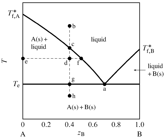
Figure 13.i Temperature–composition phase diagram for a binary system exhibiting a eutectic indicate.
Effigy 13.1 is a temperature–limerick phase diagram at a fixed pressure. The composition variable \(z\B\) is the mole fraction of component B in the system equally a whole. The phases shown are a binary liquid mixture of A and B, pure solid A, and pure solid B.
The one-phase liquid area is bounded by two curves, which we tin retrieve of either as freezing-point curves for the liquid or as solubility curves for the solids. These curves comprise the liquidus. As the mole fraction of either component in the liquid phase decreases from unity, the freezing point decreases. The curves meet at point a, which is a eutectic point. At this betoken, both solid A and solid B can coexist in equilibrium with a binary liquid mixture. The limerick at this point is the eutectic composition, and the temperature hither (denoted \(T\subs{e}\)) is the eutectic temperature. ("Eutectic" comes from the Greek for like shooting fish in a barrel melting.) \(T\subs{e}\) is the everyman temperature for the given pressure at which the liquid stage is stable.
Suppose we combine \(0.threescore\mol\) A and \(0.40\mol\) B (\(z\B=0.40\)) and suit the temperature and so every bit to put the organization bespeak at b. This point is in the i-stage liquid area, and so the equilibrium system at this temperature has a unmarried liquid phase. If we at present place the system in thermal contact with a common cold reservoir, oestrus is transferred out of the system and the arrangement indicate moves down along the isopleth (path of constant overall composition) b–h. The cooling rate depends on the temperature gradient at the system boundary and the arrangement's heat capacity.
At signal c on the isopleth, the system indicate reaches the purlieus of the one-stage surface area and is most to enter the 2-phase area labeled A(southward) + liquid. At this point in the cooling process, the liquid is saturated with respect to solid A, and solid A is about to freeze out from the liquid. There is an abrupt subtract (intermission) in the cooling rate at this bespeak, considering the freezing process involves an extra enthalpy subtract.
At the nonetheless lower temperature at signal d, the system point is within the two-phase solid–liquid area. The tie line through this point is line e–f. The compositions of the 2 phases are given past the values of \(z\B\) at the ends of the tie line: \(x\B\sups{s}=0\) for the solid and \(x\B\sups{50} =0.50\) for the liquid. From the full general lever dominion (Eq. 8.ii.8), the ratio of the amounts in these phases is \brainstorm{equation} \frac{north\sups{l} }{northward\sups{south}} = \frac{z\B-x\B\sups{s}}{x\B\sups{l} -z\B} = \frac{0.xl-0}{0.50-0.xl} = 4.0 \tag{13.ii.i} \end{equation} Since the total corporeality is \(n\sups{s}+n\sups{l} =1.00\mol\), the amounts of the two phases must be \(n\sups{southward}=0.20\mol\) and \(n\sups{50} =0.eighty\mol\).
When the system indicate reaches the eutectic temperature at signal g, cooling halts until all of the liquid freezes. Solid B freezes out as well as solid A. During this eutectic halt, there are at first three phases: liquid with the eutectic composition, solid A, and solid B. As oestrus continues to be withdrawn from the organization, the corporeality of liquid decreases and the amounts of the solids increase until finally only \(0.60\mol\) of solid A and \(0.40\mol\) of solid B are present. The temperature then begins to decrease again and the system betoken enters the ii-phase surface area for solid A and solid B; tie lines in this expanse extend from \(z\B{=}0\) to \(z\B{=}one\).
Temperature–composition stage diagrams such equally this are frequently mapped out experimentally by observing the cooling curve (temperature equally a function of time) along isopleths of various compositions. This procedure is thermal analysis. A break in the gradient of a cooling curve at a particular temperature indicates the system point has moved from a one-phase liquid area to a 2-stage area of liquid and solid. A temperature halt indicates the temperature is either the freezing bespeak of the liquid to class a solid of the same composition, or else a eutectic temperature.
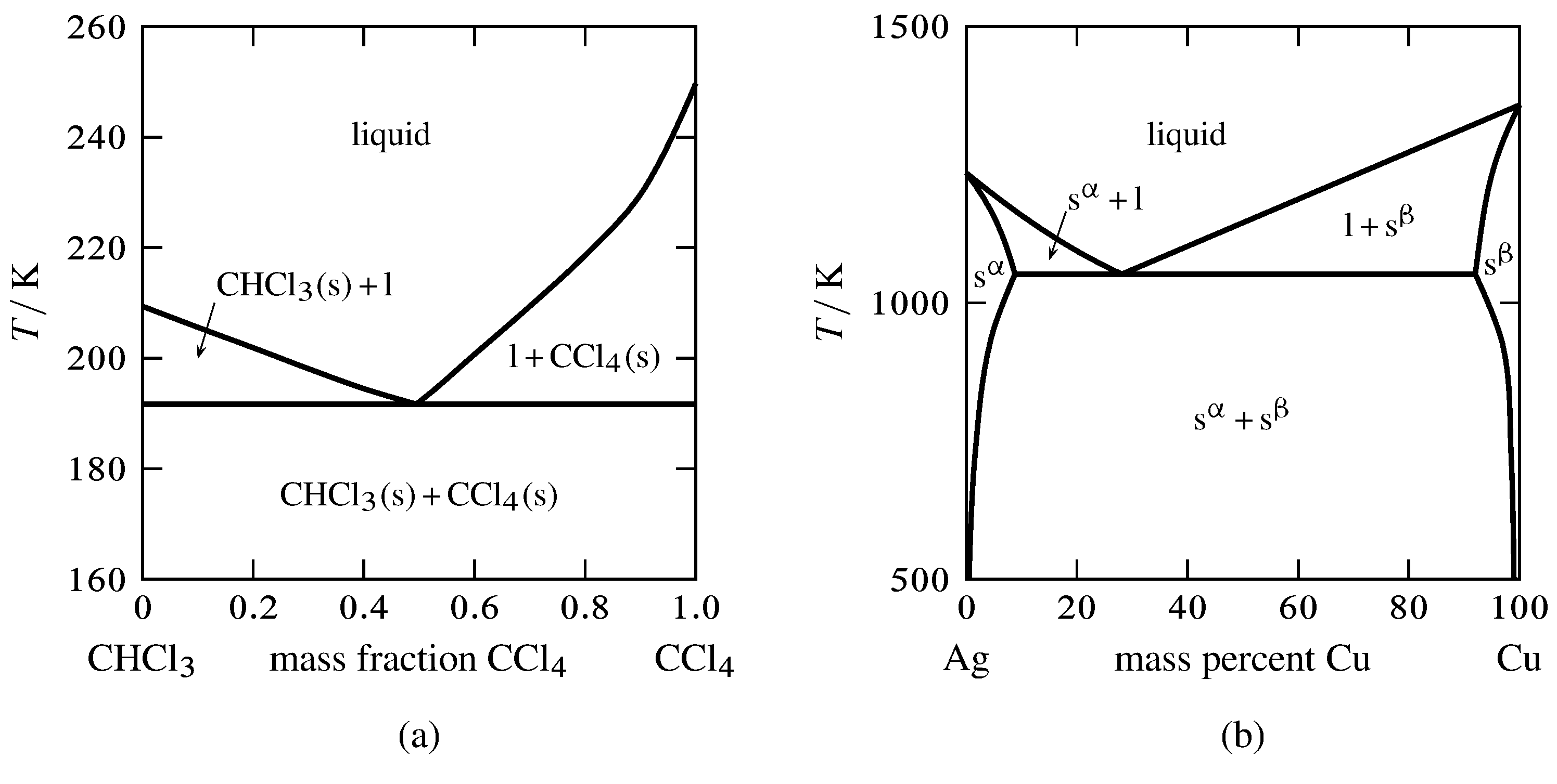
Effigy xiii.2 Temperature–limerick phase diagrams with unmarried eutectics.
(a) Two pure solids and a liquid mixture (E. Westward. Washburn, International Critical Tables of Numerical Data, Physics, Chemistry and Engineering, Vol. Four, McGraw-Loma, New York, 1928, p. 98).
(b) Two solid solutions and a liquid mixture.
Effigy 13.two shows 2 temperature–composition phase diagrams with single eutectic points. The left-manus diagram is for the binary system of chloroform and carbon tetrachloride, ii liquids that form virtually ideal mixtures. The solid phases are pure crystals, as in Fig. xiii.1. The right-hand diagram is for the silver–copper organization and involves solid phases that are solid solutions (substitutional alloys of variable composition). The area labeled due south\(\aph\) is a solid solution that is mostly silver, and s\(\bph\) is a solid solution that is mostly copper. Tie lines in the two-phase areas do not end at a vertical line for a pure solid component every bit they do in the system shown in the left-mitt diagram. The 3 phases that tin can coexist at the eutectic temperature of \(\tx{1,052}\K\) are the melt of the eutectic composition and the two solid solutions.
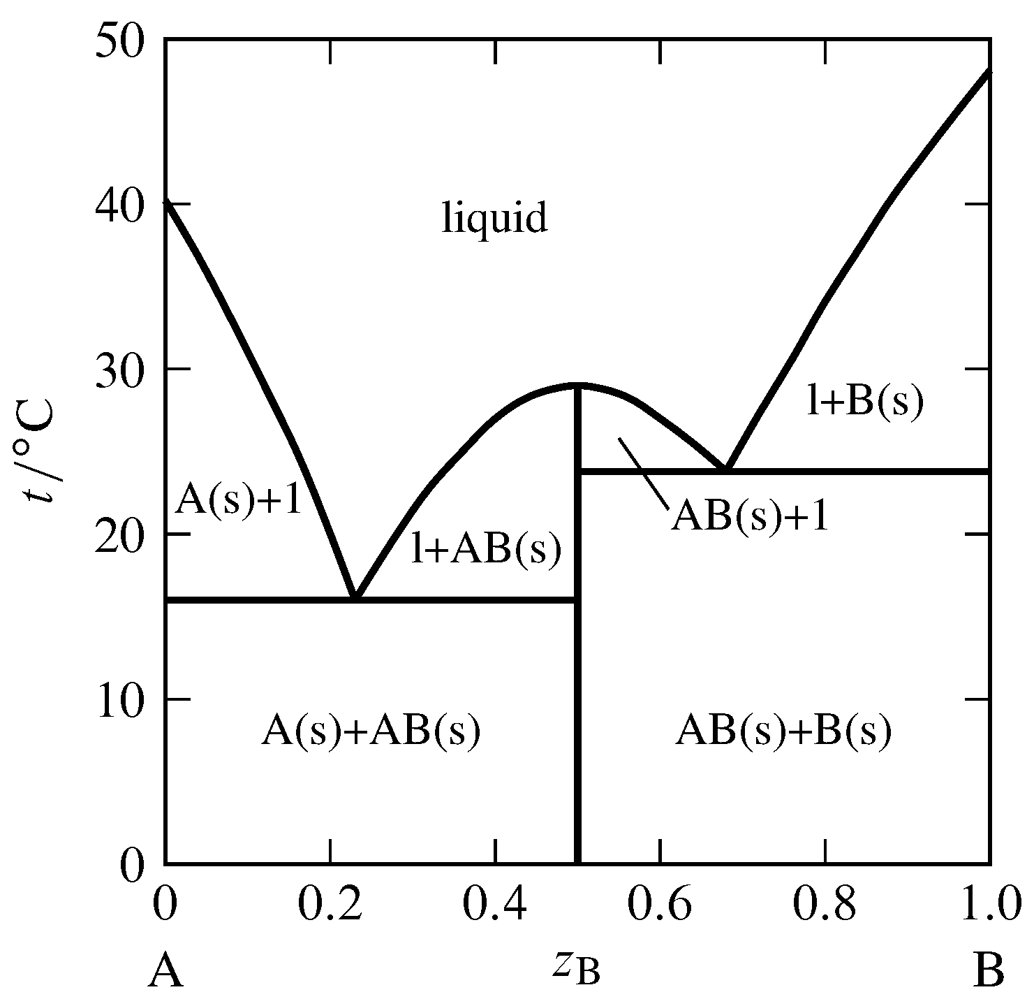
Figure 13.iii Temperature–composition phase diagram for the binary system of \(\alpha\)-naphthylamine (A) and phenol (B) at \(1\br\) (J. C. Philip, J. Chem. Soc., 83, 814–834, 1903).
Section 12.five.iv discussed the possibility of the advent of a solid compound when a binary liquid mixture is cooled. An case of this behavior is shown in Fig. 13.three, in which the solid compound contains equal amounts of the ii components \(\blastoff\)-naphthylamine and phenol. The possible solid phases are pure A, pure B, and the solid compound AB. Just one or ii of these solids can be nowadays simultaneously in an equilibrium land. The vertical line in the figure at \(z\B=0.5\) represents the solid chemical compound. The temperature at the upper end of this line is the melting point of the solid compound, \(29\units{\(\degC\)}\). The solid melts congruently to give a liquid of the aforementioned composition. A melting process with this behavior is chosen a dystectic reaction. The cooling curve for liquid of this composition would display a halt at the melting point.
The phase diagram in Fig. 13.iii has 2 eutectic points. It resembles ii unproblematic phase diagrams like Fig. 13.1 placed side by side. There is one of import deviation: the slope of the freezing-point curve (liquidus curve) is nonzero at the composition of a pure component, simply is zero at the composition of a solid compound that is completely dissociated in the liquid (as derived theoretically in Sec. 12.5.iv). Thus, the bend in Fig. 13.three has a relative maximum at the limerick of the solid compound (\(z\B=0.5\)) and is rounded at that place, instead of having a cusp—like a Romanesque arch rather than a Gothic arch.
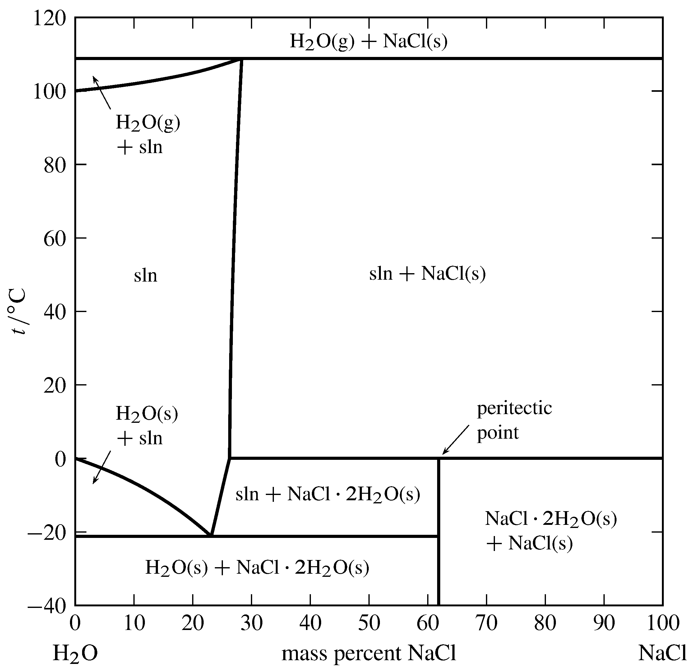
Figure 13.4 Temperature–limerick stage diagram for the binary system of H\(_2\)O and NaCl at \(1\br\). (Data from Roger Cohen-Adad and John W. Lorimer, Alkali metal and Ammonium Chlorides in Water and Heavy Water (Binary Systems), Solubility Information Series, Vol. 47, Pergamon Press, Oxford, 1991; and E. West. Washburn, International Critical Tables of Numerical Data, Physics, Chemistry and Technology, Vol. III, McGraw-Hill, New York, 1928.)
An instance of a solid compound that does not melt congruently is shown in Fig. 13.four. The solid hydrate \(\ce{NaCl*2H2O}\) is \(61.9\%\) NaCl past mass. It decomposes at \(0\units{\(\degC\)}\) to form an aqueous solution of limerick \(26.three\%\) NaCl by mass and a solid stage of anhydrous NaCl. These three phases tin coexist at equilibrium at \(0\units{\(\degC\)}\). A phase transition like this, in which a solid compound changes into a liquid and a different solid, is called incongruent or peritectic melting, and the betoken on the stage diagram at this temperature at the composition of the liquid is a peritectic point.
Figure xiii.4 shows there are two other temperatures at which three phases can be present simultaneously: \(-21\units{\(\degC\)}\), where the phases are ice, the solution at its eutectic point, and the solid hydrate; and \(109\units{\(\degC\)}\), where the phases are gaseous H\(_2\)O, a solution of composition \(28.iii\%\) NaCl by mass, and solid NaCl. Note that both segments of the right-hand purlieus of the one-phase solution area have positive slopes, significant that the solubilities of the solid hydrate and the anhydrous common salt both increase with increasing temperature.
13.2.three Partially-miscible liquids
When 2 liquids that are partially miscible are combined in certain proportions, phase separation occurs (Sec. 11.ane.6). 2 liquid phases in equilibrium with 1 another are chosen conjugate phases. Obviously the 2 phases must accept different compositions or they would be identical; the difference is called a miscibility gap. A binary system with two phases has two degrees of freedom, so that at a given temperature and pressure level each cohabit stage has a fixed composition.
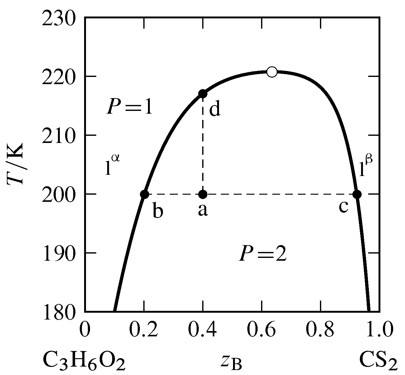
Effigy 13.5 Temperature–composition stage diagram for the binary arrangement of methyl acetate (A) and carbon disulfide (B) at \(i\br\) (data from P. Ferloni and G. Spinolo, Int. DATA Ser., Sel. Data Mixtures, Ser. A, lxx, 1974). All phases are liquids. The open circumvolve indicates the critical point.
The typical dependence of a miscibility gap on temperature is shown in Fig. 13.5. The miscibility gap (the departure in compositions at the left and right boundaries of the ii-phase expanse) decreases every bit the temperature increases until at the upper consolute temperature, also called the upper critical solution temperature, the gap vanishes. The indicate at the maximum of the purlieus curve of the two-phase expanse, where the temperature is the upper consolute temperature, is the consolute betoken or critical point. At this signal, the two liquid phases become identical, just as the liquid and gas phases get identical at the critical point of a pure substance. Critical opalescence (Sec. 8.2.3) is observed in the vicinity of this point, caused past large local limerick fluctuations. At temperatures at and in a higher place the critical bespeak, the system is a single binary liquid mixture.
Suppose we combine \(vi.0\mol\) of component A (methyl acetate) and \(4.0\mol\) of component B (carbon disulfide) in a cylindrical vessel and adjust the temperature to \(200\K\). The overall mole fraction of B is \(z\B=0.40\). The system point is at indicate a in the 2-phase region. From the positions of points b and c at the ends of the necktie line through signal a, we find the two liquid layers have compositions \(x\B\aph=0.twenty\) and \(x\B\bph=0.92\). Since carbon disulfide is the more than dense of the two pure liquids, the bottom layer is phase \(\phb\), the layer that is richer in carbon disulfide. According to the lever rule, the ratio of the amounts in the ii phases is given by \brainstorm{equation} \frac{n\bph}{n\aph} = \frac{z\B-x\B\aph}{x\B\bph-z\B} = \frac{0.40-0.twenty}{0.92-0.xl} = 0.38 \tag{13.2.2} \end{equation} Combining this value with \(n\aph+due north\bph=10.0\mol\) gives us \(n\aph=vii.ii\mol\) and \(n\bph=two.viii\mol\).
If we gradually add more than carbon disulfide to the vessel while gently stirring and keeping the temperature constant, the system point moves to the right along the tie line. Since the ends of this tie line have fixed positions, neither stage changes its composition, but the corporeality of phase \(\phb\) increases at the expense of phase \(\pha\). The liquid–liquid interface moves up in the vessel toward the meridian of the liquid cavalcade until, at overall composition \(z\B=0.92\) (bespeak c), there is just 1 liquid phase.
At present suppose the arrangement point is back at bespeak a and we raise the temperature while keeping the overall composition constant at \(z\B=0.twoscore\). The system point moves up the isopleth a–d. The phase diagram shows that the ratio \((z\B-x\B\aph)/(ten\B\bph-z\B)\) decreases during this change. Equally a result, the amount of stage \(\pha\) increases, the amount of phase \(\phb\) decreases, and the liquid–liquid interface moves down toward the bottom of the vessel until at \(217\Grand\) (bespeak d) there once again is only one liquid phase.
xiii.ii.4 Liquid–gas systems with ideal liquid mixtures
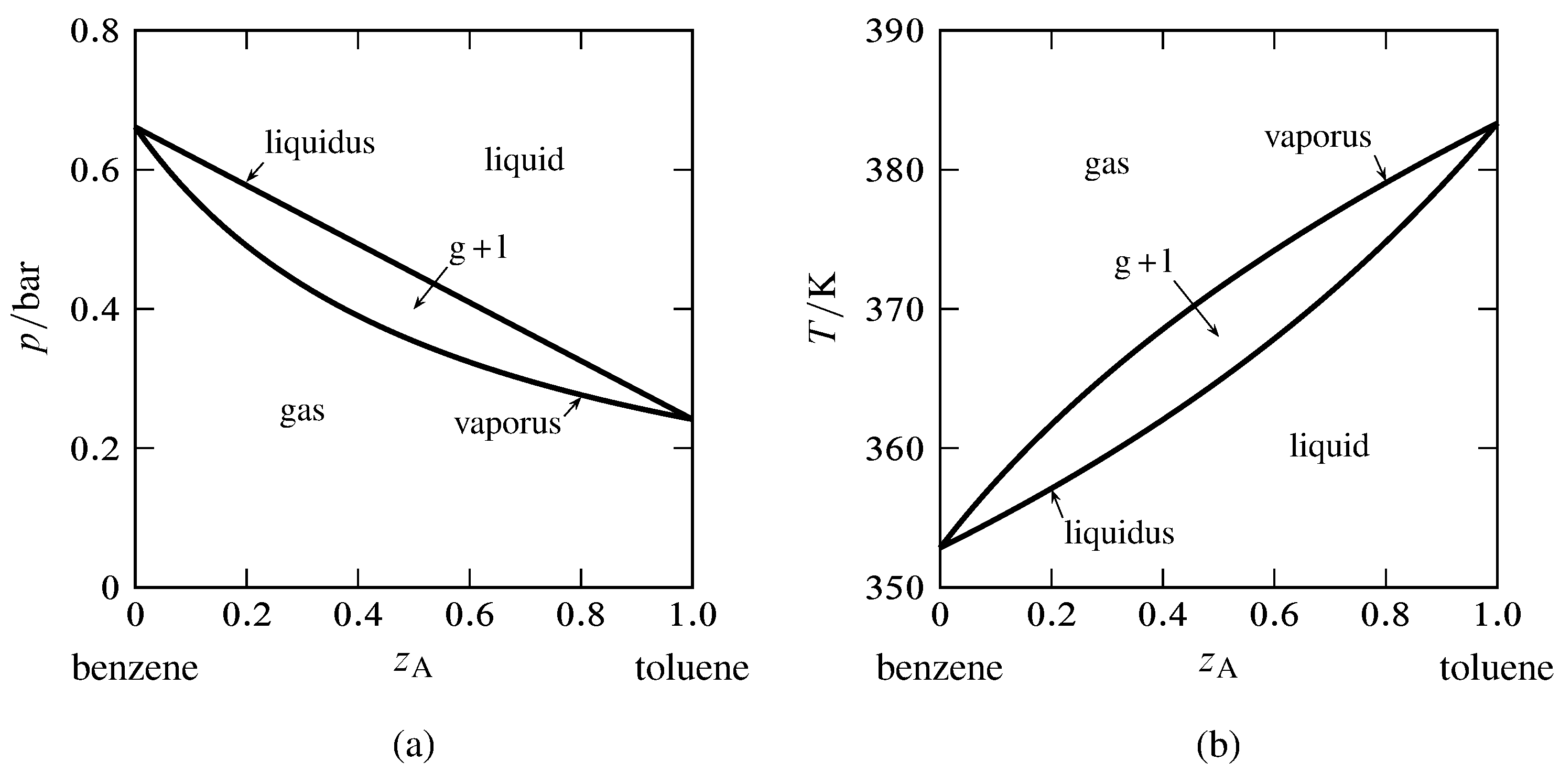
Figure xiii.6 Phase diagrams for the binary arrangement of toluene (A) and benzene (B). The curves are calculated from Eqs. 13.2.6 and 13.2.7 and the saturation vapor pressures of the pure liquids.
(a) Pressure–composition diagram at \(T=340\M\).
(b) Temperature–composition diagram at \(p=1\br\).
Toluene and benzene class liquid mixtures that are practically platonic and closely obey Raoult'southward law for partial pressure. For the binary system of these components, we can utilise the vapor pressures of the pure liquids to generate the liquidus and vaporus curves of the pressure–composition and temperature–limerick phase diagram. The results are shown in Fig. xiii.6. The composition variable \(z\A\) is the overall mole fraction of component A (toluene).
The equations needed to generate the curves can be derived equally follows. Consider a binary liquid mixture of components A and B and mole fraction composition \(x\A\) that obeys Raoult'southward law for fractional force per unit area (Eq. nine.4.2): \begin{equation} p\A = ten\A p\A^* \qquad p\B = (1-x\A)p\B^* \tag{thirteen.2.3} \terminate{equation} Strictly speaking, Raoult'due south police applies to a liquid–gas system maintained at a constant force per unit area by means of a third gaseous component, and \(p\A^*\) and \(p\B^*\) are the vapor pressures of the pure liquid components at this pressure and the temperature of the arrangement. However, when a liquid phase is equilibrated with a gas phase, the partial pressure of a constituent of the liquid is practically independent of the full pressure (Sec. 12.8.1), and so that it is a good approximation to apply the equations to a binary liquid–gas system and care for \(p\A^*\) and \(p\B^*\) as functions only of \(T\).
When the binary system contains a liquid phase and a gas stage in equilibrium, the pressure is the sum of \(p\A\) and \(p\B\), which from Eq. xiii.2.3 is given by \begin{gather} \s {\begin{split up} p & = 10\A p\A^* + (1-x\A)p\B^* \cr & = p\B^* + (p\A^*-p\B^*)10\A \end{split} } \tag{13.2.four} \cond{(\(C{=}2\), ideal liquid mixture)} \end{gather} where \(x\A\) is the mole fraction of A in the liquid phase. Equation 13.2.four shows that in the two-phase organization, \(p\) has a value between \(p\A^*\) and \(p\B^*\), and that if \(T\) is constant, \(p\) is a linear part of \(10\A\). The mole fraction composition of the gas in the two-stage system is given by \begin{equation} y\A = \frac{p\A}{p} = \frac{ten\A p\A^*}{p\B^* + (p\A^*-p\B^*)x\A } \tag{13.2.v} \finish{equation}
A binary two-stage organisation has two degrees of freedom. At a given \(T\) and \(p\), each stage must have a fixed composition. We can calculate the liquid limerick past rearranging Eq. 13.2.4: \begin{gather} \s {x\A = \frac{p-p\B^*}{p\A^*-p\B^*}} \tag{xiii.2.6} \cond{(\(C{=}two\), ideal liquid mixture)} \end{get together} The gas composition is and then given past \begin{gather} \s {\brainstorm{split} y\A & = \frac{p\A}{p} = \frac{x\A p\A^*}{p} \cr & = \left( \frac{p-p\B^*}{p\A^*-p\B^*}\right) \frac{p\A^*}{p} \end{split} } \tag{13.two.7} \cond{(\(C{=}2\), ideal liquid mixture)} \end{get together}
If we know \(p\A^*\) and \(p\B^*\) every bit functions of \(T\), nosotros can use Eqs. 13.two.6 and 13.2.7 to calculate the compositions for any combination of \(T\) and \(p\) at which the liquid and gas phases tin coexist, and thus construct a pressure–limerick or temperature–composition phase diagram.
In Fig. thirteen.half dozen(a), the liquidus bend shows the relation between \(p\) and \(x\A\) for equilibrated liquid and gas phases at abiding \(T\), and the vaporus curve shows the relation between \(p\) and \(y\A\) under these atmospheric condition. We see that \(p\) is a linear office of \(x\A\) but not of \(y\A\).
In a like fashion, the liquidus curve in Fig. 13.6(b) shows the relation between \(T\) and \(x\A\), and the vaporus bend shows the relation between \(T\) and \(y\A\), for equilibrated liquid and gas phases at constant \(p\). Neither curve is linear.
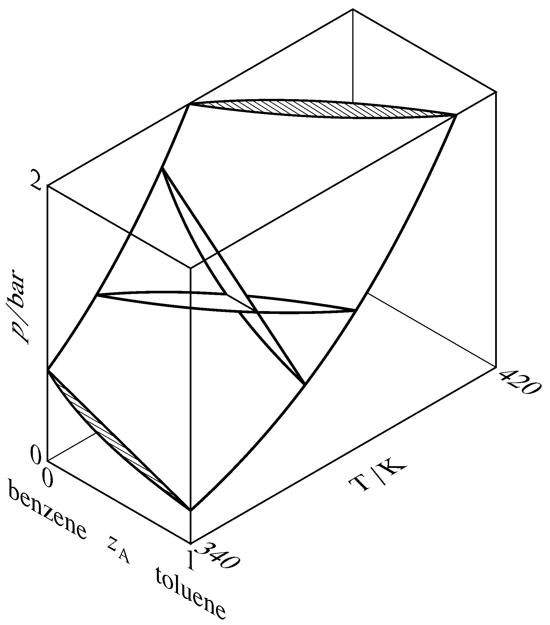
Figure 13.7 Liquidus and vaporus surfaces for the binary organization of toluene (A) and benzene. Cantankerous-sections through the two-phase region are drawn at constant temperatures of \(340\K\) and \(370\K\) and at constant pressures of \(1\br\) and \(2\br\). 2 of the cross-sections intersect at a tie line at \(T=370\1000\) and \(p=ane\br\), and the other cross-sections are hatched in the direction of the tie lines.
A liquidus bend is besides called a chimera-point bend or a boiling-point bend. Other names for a vaporus curve are dew-point curve and condensation curve. These curves are really cross-sections of liquidus and vaporus surfaces in a three-dimensional \(T\)–\(p\)–\(z\A\) phase diagram, equally shown in Fig. xiii.7. In this figure, the liquidus surface is in view at the front and the vaporus surface is hidden behind information technology.
thirteen.2.5 Liquid–gas systems with nonideal liquid mixtures
Most binary liquid mixtures practice not bear ideally. The most mutual situation is positive deviations from Raoult's law. (In the molecular model of Sec. 11.i.5, positive deviations correspond to a less negative value of \(k\subs{AB}\) than the average of \(k\subs{AA}\) and \(k\subs{BB}\).) Some mixtures, however, accept specific A–B interactions, such every bit solvation or molecular clan, that foreclose random mixing of the molecules of A and B, and the result is and then negative deviations from Raoult'south law. If the deviations from Raoult's law, either positive or negative, are large enough, the constant-temperature liquidus curve exhibits a maximum or minimum and azeotropic beliefs results.
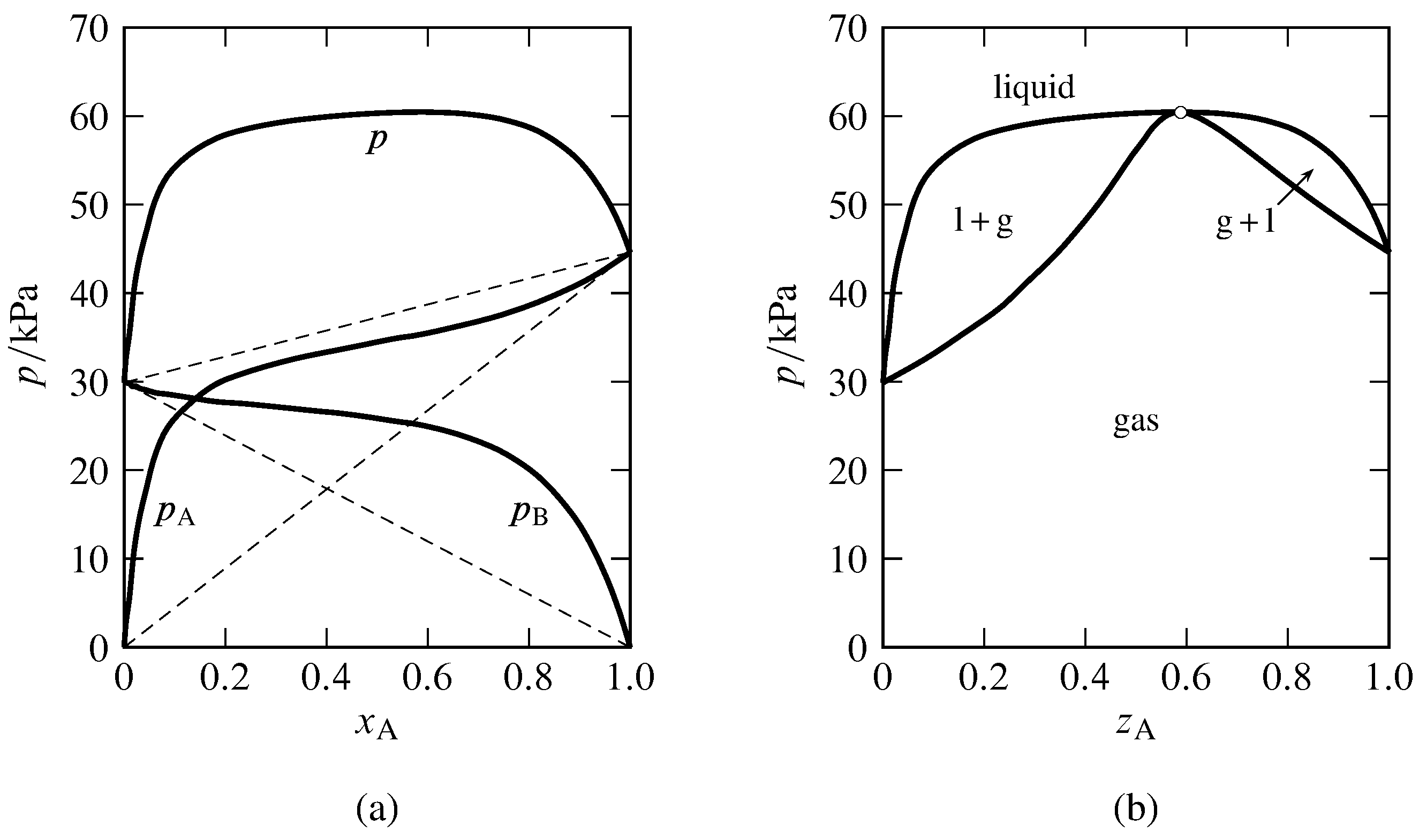
Figure 13.eight Binary arrangement of methanol (A) and benzene at \(45\units{\(\degC\)}\) (Hossein Toghiani, Rebecca K. Toghiani, and Dabir Southward. Viswanath, J. Chem. Eng. Data, 39, 63–67, 1994).
(a) Partial pressures and total pressure in the gas stage equilibrated with liquid mixtures. The dashed lines indicate Raoult'south law behavior.
(b) Pressure level–composition stage diagram at \(45\units{\(\degC\)}\). Open circle: azeotropic betoken at \(z\A=0.59\) and \(p=60.5\units{kPa}\).
Figure 13.eight shows the azeotropic beliefs of the binary methanol-benzene system at constant temperature. In Fig. xiii.8(a), the experimental fractional pressures in a gas phase equilibrated with the nonideal liquid mixture are plotted every bit a function of the liquid composition. The partial pressures of both components exhibit positive deviations from Raoult'southward law, consequent with the statement in Sec. 12.eight.two that if i constituent of a binary liquid mixture exhibits positive deviations from Raoult's police, with only ane inflection point in the bend of fugacity versus mole fraction, the other constituent also has positive deviations from Raoult's constabulary. The total pressure (equal to the sum of the fractional pressures) has a maximum value greater than the vapor pressure of either pure component. The bend of \(p\) versus \(x\A\) becomes the liquidus curve of the force per unit area–composition phase diagram shown in Fig. 13.8(b). Points on the vaporus curve are calculated from \(p=p\A/y\A\).
In practise, the data needed to generate the liquidus and vaporus curves of a nonideal binary organization are commonly obtained by assuasive liquid mixtures of various compositions to eddy in an equilibrium still at a fixed temperature or pressure. When the liquid and gas phases have become equilibrated, samples of each are withdrawn for analysis. The partial pressures shown in Fig. 13.8(a) were calculated from the experimental gas-phase compositions with the relations \(p\A=y\A p\) and \(p\B=p-p\A\).
If the abiding-temperature liquidus bend has a maximum pressure at a liquid composition non corresponding to one of the pure components, which is the case for the methanol–benzene system, then the liquid and gas phases are mixtures of identical compositions at this pressure. This behavior was deduced at the end of Sec. 12.eight.iii. On the pressure level–composition stage diagram, the liquidus and vaporus curves both accept maxima at this pressure, and the two curves coincide at an azeotropic point. A binary arrangement with negative deviations from Raoult'south constabulary can take an isothermal liquidus curve with a minimum pressure at a particular mixture composition, in which example the liquidus and vaporus curves coincide at an azeotropic point at this minimum. The general phenomenon in which equilibrated liquid and gas mixtures have identical compositions is called azeotropy, and the liquid with this composition is an azeotropic mixture or azeotrope (Greek: boils unchanged). An azeotropic mixture vaporizes equally if information technology were a pure substance, undergoing an equilibrium stage transition to a gas of the aforementioned composition.
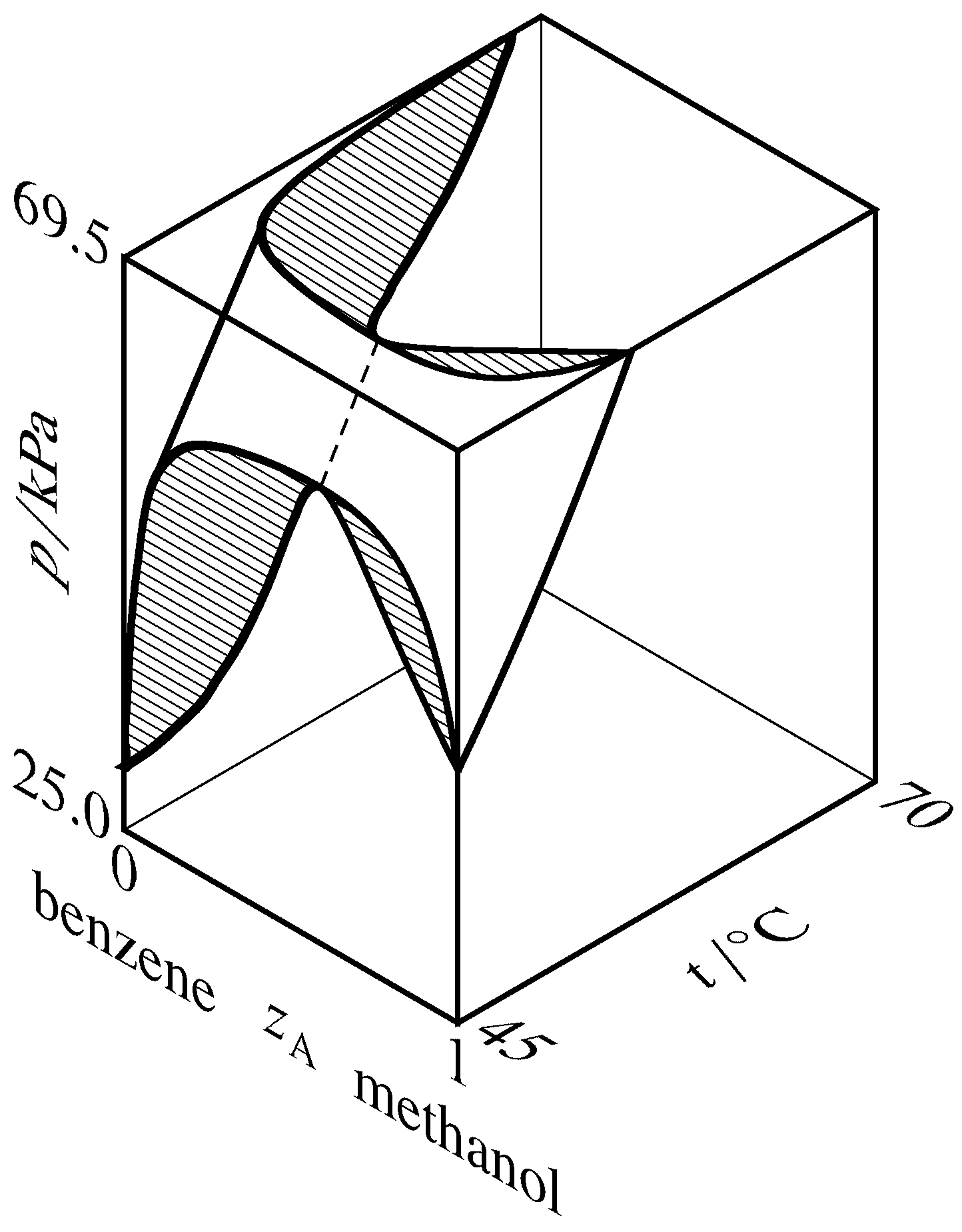
Figure 13.9 Liquidus and vaporus surfaces for the binary arrangement of methanol (A) and benzene (Hossein Toghiani, Rebecca Thou. Toghiani, and Dabir South. Viswanath, J. Chem. Eng. Data, 39, 63–67, 1994). Cross-sections are hatched in the direction of the tie lines. The dashed curve is the azeotrope vapor-pressure level bend.
If the liquidus and vaporus curves exhibit a maximum on a pressure–composition phase diagram, so they showroom a minimum on a temperature–composition stage diagram. This relation is explained for the methanol–benzene organisation past the iii-dimensional liquidus and vaporus surfaces fatigued in Fig. 13.9. In this diagram, the vaporus surface is subconscious behind the liquidus surface. The hatched cross-section at the front of the figure is the aforementioned as the pressure–composition diagram of Fig. 13.8(b), and the hatched cross-section at the elevation of the figure is a temperature–composition phase diagram in which the system exhibits a minimum-humid azeotrope.
A binary system containing an azeotropic mixture in equilibrium with its vapor has 2 species, two phases, and one relation among intensive variables: \(x\A =y\A\). The number of degrees of freedom is and then \(F = two+s-r-P = 2+ii-1-2 = 1\); the system is univariant. At a given temperature, the azeotrope tin be at only one pressure and have merely one composition. Every bit \(T\) changes, and so do \(p\) and \(z\A\) forth an azeotrope vapor-pressure bend as illustrated by the dashed curve in Fig. 13.9.
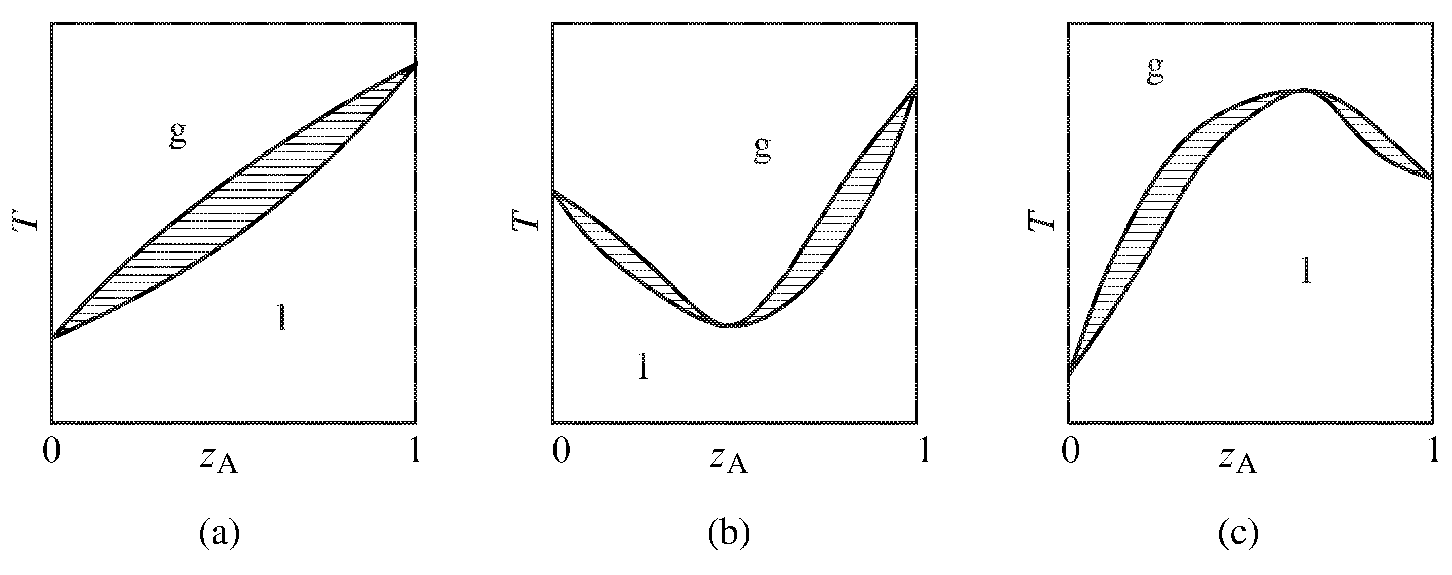
Figure xiii.x Temperature–composition phase diagrams of binary systems exhibiting (a) no azeotropy, (b) a minimum-boiling azeotrope, and (c) a maximum-humid azeotrope. Only the one-phase areas are labeled; two-phase areas are hatched in the direction of the tie lines.
Figure 13.10 summarizes the general appearance of some relatively uncomplicated temperature–composition stage diagrams of binary systems. If the organisation does not form an azeotrope (zeotropic behavior), the equilibrated gas phase is richer in one component than the liquid stage at all liquid compositions, and the liquid mixture can exist separated into its two components past fractional distillation. The gas in equilibrium with an azeotropic mixture, however, is not enriched in either component. Partial distillation of a system with an azeotrope leads to separation into one pure component and the azeotropic mixture.
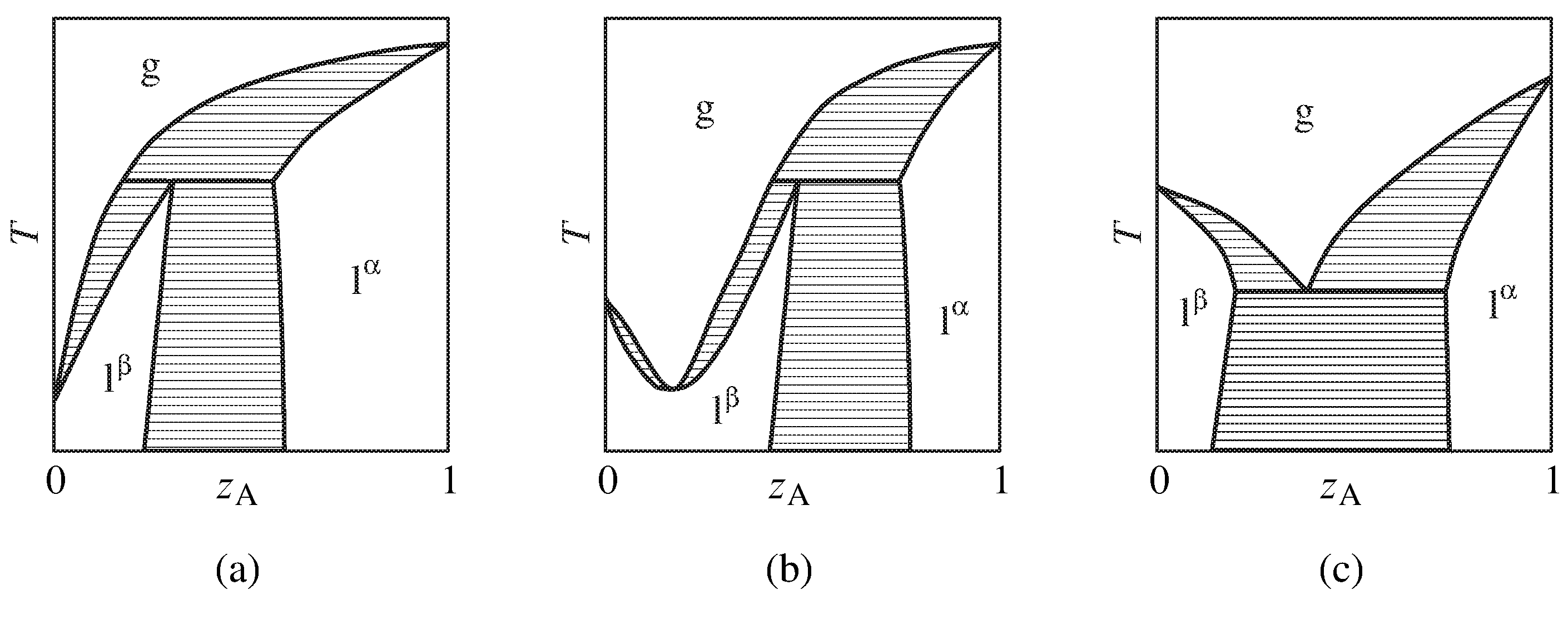
Figure xiii.eleven Temperature–composition stage diagrams of binary systems with partially-miscible liquids exhibiting (a) the ability to exist separated into pure components by partial distillation, (b) a minimum-boiling azeotrope, and (c) boiling at a lower temperature than the boiling point of either pure component. Simply the one-phase areas are labeled; two-phase areas are hatched in the direction of the tie lines.
More complicated beliefs is shown in the stage diagrams of Fig. 13.xi. These are binary systems with partially-miscible liquids in which the boiling indicate is reached before an upper consolute temperature tin can be observed.
13.2.6 Solid–gas systems
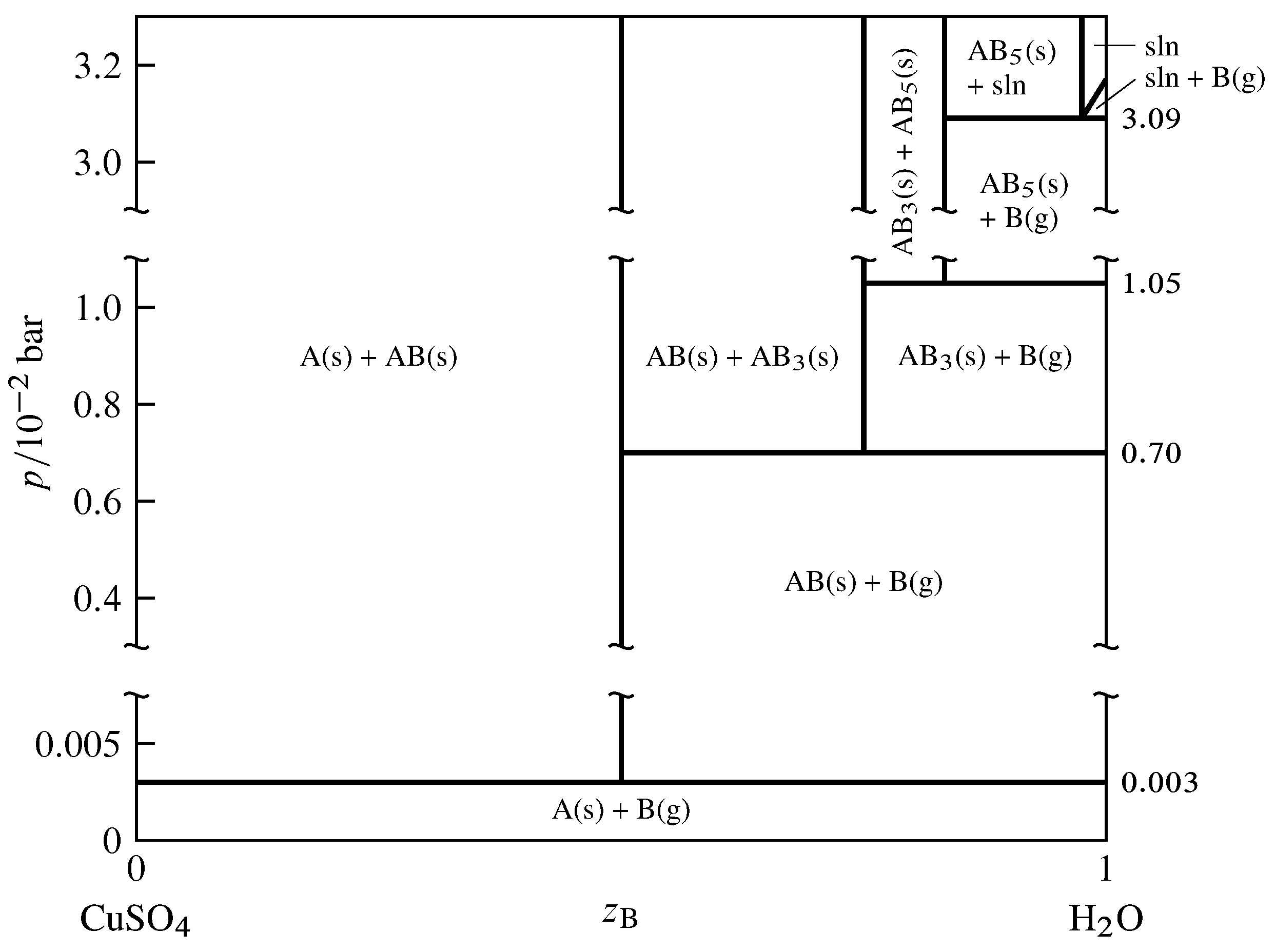
Effigy 13.12 Pressure–composition stage diagram for the binary organisation of CuSO\(_4\) (A) and H\(_2\)O (B) at \(25\units{\(\degC\)}\) (Thomas S. Logan, J. Chem. Educ., 35, 148–149, 1958; Due east. W. Washburn, International Critical Tables of Numerical Data, Physics, Chemical science and Engineering science, Vol. VII, McGraw-Hill, New York, 1930, p. 263).
Every bit an example of a two-component arrangement with equilibrated solid and gas phases, consider the components \(\ce{CuSO4}\) and \(\ce{H2O}\), denoted A and B respectively. In the pressure–limerick phase diagram shown in Fig. 13.12, the limerick variable \(z\B\) is every bit usual the mole fraction of component B in the system as a whole.
The anhydrous salt and its hydrates (solid compounds) form the series of solids \(\ce{CuSO4}\), \(\ce{CuSO4*H2o}\), \(\ce{CuSO4*3H2O}\), and \(\ce{CuSO4*5H2O}\). In the phase diagram these formulas are abbreviated A, AB, AB\(_3\), and AB\(_5\). The following dissociation equilibria (dehydration equilibria) are possible: \begin{align*} \ce{CuSO4*H2o}\tx{(s)} & \arrows \ce{CuSO4}\tx{(south)} + \ce{H2O}\tx{(k)}\cr \ce{i/2CuSO4*3H2O}\tx{(s)} & \arrows \ce{one/2CuSO4*H2O}\tx{(s)} + \ce{H2O}\tx{(k)}\cr \ce{one/2CuSO4*5H2O}\tx{(southward)} & \arrows \ce{i/2CuSO4*3H2O}\tx{(s)} + \ce{H2o}\tx{(yard)} \finish{marshal*} The equilibria are written above with coefficients that make the coefficient of H\(_2\)O(k) unity. When 1 of these equilibria is established in the system, in that location are two components and three phases; the phase dominion then tells us the system is univariant and the pressure level has only one possible value at a given temperature. This pressure is called the dissociation force per unit area of the higher hydrate.
The dissociation pressures of the three hydrates are indicated by horizontal lines in Fig. thirteen.12. For example, the dissociation pressure of \(\ce{CuSO4*5H2O}\) is \(1.05\timesten{-two}\units{\(\br\)}\). At the pressure of each horizontal line, the equilibrium system can have one, ii, or 3 phases, with compositions given past the intersections of the line with vertical lines. A fourth three-stage equilibrium is shown at \(p=3.09\timesten{-2}\units{\(\br\)}\); this is the equilibrium between solid \(\ce{CuSO4*5H2O}\), the saturated aqueous solution of this hydrate, and water vapor.
Consider the thermodynamic equilibrium constant of ane of the dissociation reactions. At the depression pressures shown in the phase diagram, the activities of the solids are practically unity and the fugacity of the water vapor is practically the aforementioned every bit the force per unit area, so the equilibrium abiding is almost exactly equal to \(p\subs{d}/p\st\), where \(p\subs{d}\) is the dissociation pressure of the higher hydrate in the reaction. Thus, a hydrate cannot exist in equilibrium with h2o vapor at a pressure below the dissociation pressure of the hydrate because dissociation would be spontaneous nether these conditions. Conversely, the common salt formed by the dissociation of a hydrate cannot exist in equilibrium with h2o vapor at a pressure level in a higher place the dissociation pressure because hydration would be spontaneous.
If the system contains dry air every bit an additional gaseous component and one of the dissociation equilibria is established, the fractional pressure \(p\subs{H\(_2\)O}\) of H\(_2\)O is equal (approximately) to the dissociation pressure level \(p\subs{d}\) of the higher hydrate. The prior statements regarding dissociation and hydration now depend on the value of \(p\subs{H\(_2\)O}\). If a hydrate is placed in air in which \(p\subs{H\(_2\)O}\) is less than \(p\subs{d}\), dehydration is spontaneous; this phenomenon is chosen efflorescence (Latin: blossoming). If \(p\subs{H\(_2\)O}\) is greater than the vapor force per unit area of the saturated solution of the highest hydrate that can form in the system, the anhydrous common salt and whatsoever of its hydrates will spontaneously blot water and class the saturated solution; this is deliquescence (Latin: becoming fluid).
If the 2-component equilibrium system contains only ii phases, information technology is bivariant corresponding to one of the areas in Fig. 13.12. Hither both the temperature and the pressure can be varied. In the case of areas labeled with two solid phases, the pressure has to be applied to the solids by a fluid (other than H\(_2\)O) that is not considered part of the system.
13.2.7 Systems at high pressure
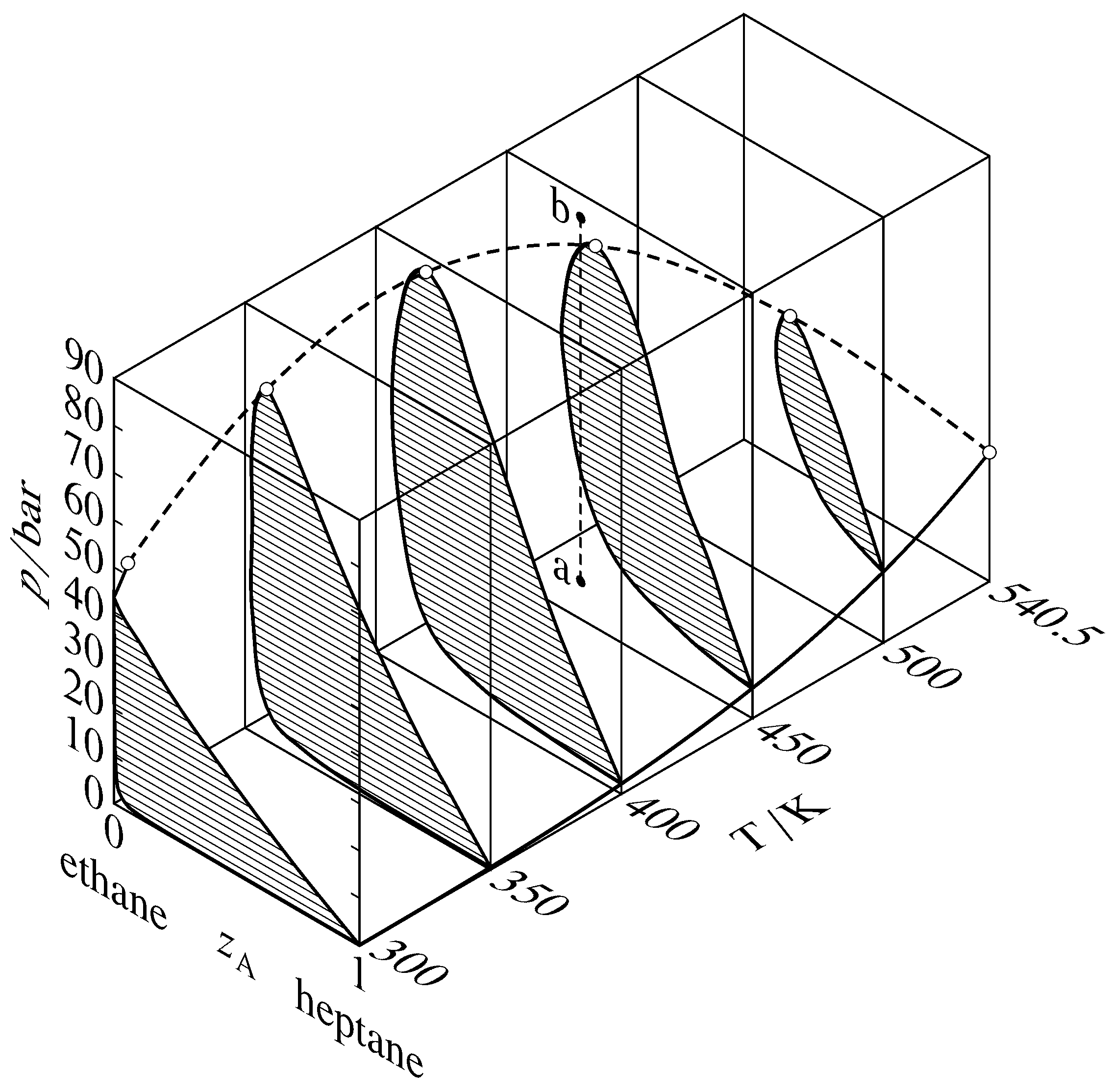
Figure 13.thirteen Pressure–temperature–composition behavior in the binary heptane–ethane system (W. B. Kay, Ind. Eng. Chem., thirty, 459–465, 1938). The open circles are critical points; the dashed curve is the critical bend. The dashed line a–b illustrates retrograde condensation at \(450\One thousand\).
Binary phase diagrams brainstorm to look different when the force per unit area is greater than the disquisitional pressure level of either of the pure components. Various types of behavior accept been observed in this region. One mutual type, that institute in the binary system of heptane and ethane, is shown in Fig. 13.13. This effigy shows sections of a iii-dimensional phase diagram at 5 temperatures. Each section is a pressure–composition phase diagram at constant \(T\). The two-stage areas are hatched in the direction of the tie lines. At the left end of each tie line (at low \(z\A\)) is a vaporus curve, and at the right cease is a liquidus curve. The vapor pressure level curve of pure ethane (\(z\A{=}0\)) ends at the disquisitional point of ethane at \(305.4\K\); between this point and the critical point of heptane at \(540.five\K\), there is a continuous critical curve, which is the locus of disquisitional points at which gas and liquid mixtures go identical in composition and density.
Consider what happens when the system betoken is at point a in Fig. 13.thirteen and the pressure is then increased by isothermal compression along line a–b. The system bespeak moves from the area for a gas phase into the two-phase gas–liquid surface area and then out into the gas-stage area over again. This curious phenomenon, condensation followed by vaporization, is called retrograde condensation.
Under some conditions, an isobaric increase of \(T\) tin result in vaporization followed by condensation; this is retrograde vaporization.

Effigy 13.xiv Pressure–temperature–composition behavior in the binary xenon–helium arrangement (J. de Swann Arons and Yard. A. 1000. Diepen, J. Chem. Phys., 44, 2322–2330, 1966). The open circles are disquisitional points; the dashed curve is the disquisitional curve.
A different blazon of high-pressure behavior, that found in the xenon–helium system, is shown in Fig. 13.14. Hither, the critical curve begins at the disquisitional point of the less volatile component (xenon) and continues to college temperatures and pressures than the disquisitional temperature and pressure of either pure component. The ii-phase region at pressures above this critical curve is sometimes said to stand for gas–gas equilibrium, or gas–gas immiscibility, because we would not usually consider a liquid to be beyond the critical points of the pure components. Of class, the coexisting phases in this two-phase region are non gases in the ordinary sense of existence tenuous fluids, but are instead loftier-pressure fluids of liquid-like densities. If we want to call both phases gases, then we have to say that pure gaseous substances at high pressure do not necessarily mix spontaneously in all proportions as they exercise at ordinary pressures.
If the pressure of a organization is increased isothermally, eventually solid phases volition appear; these are not shown in Figs. 13.13 and Fig. 13.14.
Source: https://chem.libretexts.org/Bookshelves/Physical_and_Theoretical_Chemistry_Textbook_Maps/DeVoes_Thermodynamics_and_Chemistry/13:_The_Phase_Rule_and_Phase_Diagrams/13.02:__Phase_Diagrams-_Binary_Systems
0 Response to "How to Read Tie Line on Equilibrium Phase Diagram"
Post a Comment